Introduction to Approximate Bayesian Computation (ABC)
In population genetics and gene drive modeling, parameter estimation can be extremely difficult with complex situations. In these models, the likelihood function is typically intractable, meaning it is difficult or impossible to write down in a closed form due to stochasticity, high-dimensional parameter spaces, and non-linear genotype dynamics. Traditional likelihood-based inference methods are therefore often impractical.
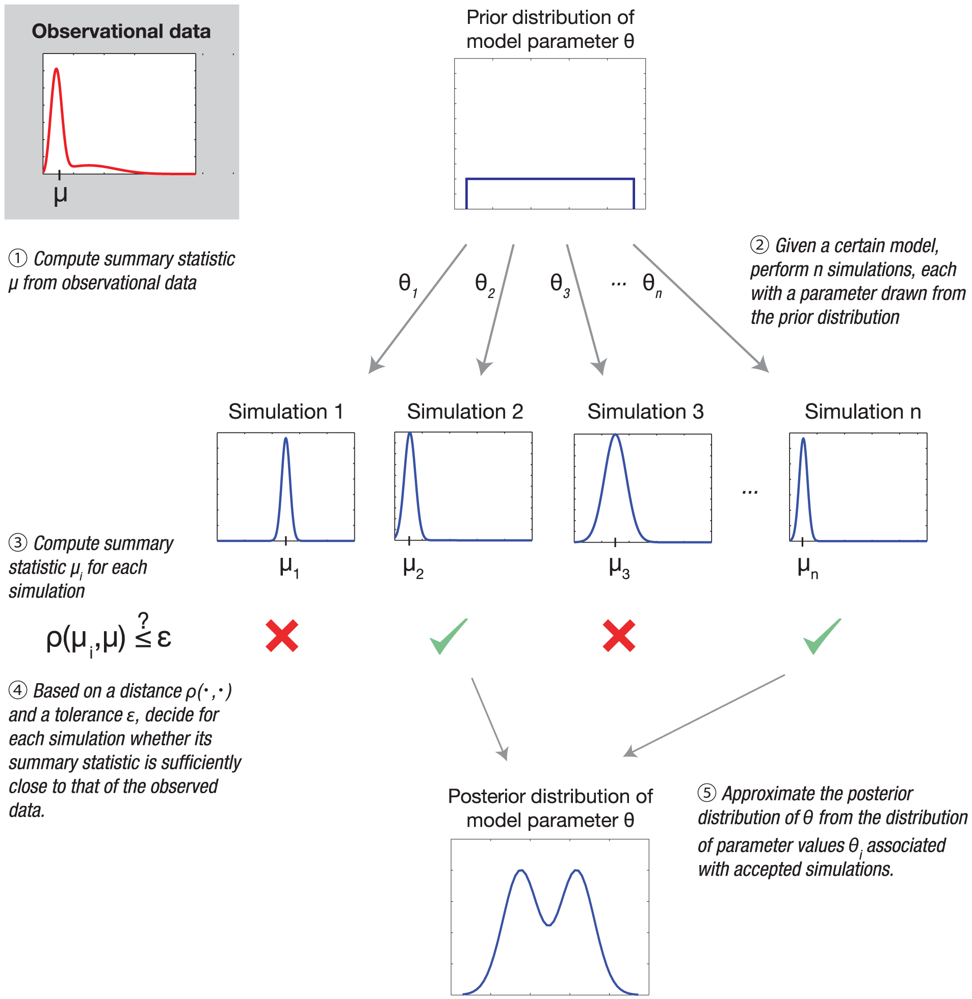
Approximate Bayesian Computation (ABC) provides a likelihood-free framework to estimate parameters by comparing simulated data from the model to observed data. The basic idea is to accept parameter values that produce simulated outputs sufficiently close to the observations, forming an approximate posterior distribution for the parameters of interest. The general ABC procedure is as follows:
- Sample parameters $\theta$ from the prior distribution $p(\theta)$.
- Simulate genotype trajectories $g_{\text{sim}}$ from the evolutionary model using $\theta$.
- Compare the simulated data $g_{\text{sim}}$ to the observed data $g_{\text{obs}}$ using a distance metric $d(g_{\text{sim}}, g_{\text{obs}})$.
- Accept $\theta$ if $d \le \epsilon$, where $\epsilon$ is a predefined tolerance.
- Repeat steps 2–4. The collection of accepted $\theta$ values forms an approximate posterior $p(\theta \mid g_{\text{obs}})$.
While ABC is conceptually simple, it can be computationally expensive because simulating the model for every sampled parameter combination in high-dimensional spaces can be prohibitive. To address this challenge, Sequential Monte Carlo (SMC) can be combined with ABC to form the ABC-SMC algorithm, which gradually refines the particle population toward regions of high posterior probability in an adaptive manner:
- Initialize a population of particles ${\theta^{(i)}_0}$ sampled from the prior $p(\theta)$.
- At iteration $t$, simulate genotype trajectories ${g_{\text{sim},t}^{(i)}}$ for each particle and accept those with distances $d \le \epsilon_t$.
-
Compute particle weights based on distances:
\[w^{(i)}_t = \begin{cases} 1, & t=0, \\ \dfrac{p(\theta_t^{(i)})}{\sum_{j=1}^{N} w^{(j)}_{t-1} K_t(\theta_{t-1}^{(j)}, \theta_t^{(i)})}, & t>0. \end{cases}\] - Resample particles with small Gaussian perturbations $K_{t+1}(\theta \mid \theta_t^\ast) \sim \mathcal{N}(\theta_t^\ast, \sigma^2)$ based on their weights to form the new population ${\theta^{(i)}_{t+1}}$.
- Repeat steps 2–4 for multiple iterations (e.g., 15) to reach sufficient effective sample size (ESS) and gradually reduce the tolerance $\epsilon_t$.
- The final set of particles represents an approximate posterior distribution of the fitness parameters.
By combining ABC with SMC, this method provides a practical and efficient approach to infer parameters in complex, stochastic population models, enabling researchers to capture the evolutionary dynamics of gene drives while accounting for uncertainty and variability in the system.